Quick start

Dependencies

Kestrel is written in Fortran 2003, with some additional C++ calls to geospatial libraries. It should be possible to compile and run it on most modern Unix-like platforms relatively painlessly. In order to do so, make sure the following dependencies are present on your system:

• Either GCC version 9+, or an older GCC plus the Boost C++ libraries (>= 1.46.0)

• GDAL (>= 2.2.0)

• PROJ

• GNU autotools (if building directly from the git repository)

• (optional) NetCDF (the NetCDF-Fortran library is required in this case)

• (optional) Julia, for running tests

On GNU/Linux/UNIX systems, these should be available via your package manager. For MacOS users, we recommend installing these dependencies with homebrew.

Installation

We use GNU autotools for our build system. If building directly from the git repository, you must first generate the relevant build scripts using the command

$ autoreconf -fi

Then the code can be compiled with

$ ./configure && make

If successful, this places an executable in the src directory. Alternatively, you may wish to install Kestrel in another location with the commands:

$ ./configure --prefix=[installation-directory] && make && make install

It is sometimes necessary to provide additional flags to the configure script, depending on your local setup. For example, you can do

$ ./configure --with-netcdf4=yes/no/PATH

to specify whether to build Kestrel with NetCDF support, where PATH is the base directory of your (serial) NetCDF installation. Since NetCDF is useful (and preferred) we build this support in, if found, unless otherwise specified.

Likewise, if you do not have a newer (>= 9) version of GCC, you can instead use Boost to do filesystem calls by specifying

$ ./configure --with-boost[=ARG]

where ARG optionally specifies the location of your Boost installation.

Both the GDAL and PROJ libraries are required and sometimes might be in unusual places, depending on your system. If they are not found automatically, their base directories can be specified with

$ ./configure --with-gdal=[ARG] --with-proj=[ARG]

For testing, the path to a valid Julia executable can be specified with

$ ./configure JULIA=[PATH]

This will place a symlink to Julia in the ./tests directory.

Some other options are listed in the help dialogue of the configure script

$ ./configure --help

Running simulations

Kestrel is run on the command line by specifying a text file containing the required settings and parameters for the simulations. We have provided a couple of correctly formatted input files to get you started in the examples/ directory.

1D example

To begin with, we shall set up a simple simulation of an initial release of turbulent water, propagating down an inerodible constant slope.

Input file

Take a look at the file examples/Input1d_cap_constslope.txt. You should see some settings fields divided into conceptual blocks. Let’s go through these in turn.

First is the Domain block, which sets up the simulation area.

Domain:
Lat = 0
Lon = 0
nXtiles = 6
nYtiles = 1
nXpertile = 200
nYpertile = 1
Xtilesize = 200

The domain is a rectangular region centred at the coordinates specified by Lat and Lon. It is partitioned into 6 tiles in the \(x\) direction. Each of these tiles is further subdivided into nXpertile = 200 finite volumes. Since this is a 1D simulation, the corresponding parameters in the \(y\) direction are set to 1. The final variable sets the width in metres of each tile. This implies that the resolution of the numerical discretisation is Xtilesize / nXpertile = 1 metre.

Next, the Cap block sets an initial release of flowing material.

Cap:
capX = -200
capRadius = 50
capHeight = 5
capU = 3.0
capConc = 0.0
capShape = flat

This is a volume of radius 50m, height 5m, initial horizontal velocity 3m/s and zero solids, centred at \(x = -200\)m.

The Topog block describes the initial topographic surface over which the flow propagates.

Topog:
Type = Function
Topog function = xSlope
Topog params = (-0.04)

In this case, a constant slope with gradient -0.04 (in \(x\)). Topog params is a list that can specify multiple parameters (if required) for more complicated topographies.

The Parameters block declares settings that affect the model equations, such as certain constants, closure functions and other choices.

Parameters:
Drag = Chezy
Chezy Co = 0.04
Erosion = Off

Here, we specified that we want to use the commonplace Chézy (or turbulent fluid) drag law, give the drag coefficient, 0.04, and turn erosion off.

Next are the Solver settings, which specify further arguments for the numerical method.

Solver:
T end = 100
cfl = 0.5

In particular this includes the length of time to simulate for (100 seconds). The last line provides the CFL condition for the solver, which is used to adaptively limit the time step. This normally defaults to 0.25, but in 1D, a higher value may be used.

Finally, the Output block requests 4 simulation outputs. These will be separated by equal time intervals of \(\Delta T = 100 / 4\) seconds and placed in the specified directory.

Output:
N out = 4
directory = 1d_cap_constslope/

We can run the simulation from within the examples/ directory using the command

$ ../src/kestrel Input1d_cap_constslope.txt

You can find the output in examples/1d_cap_constslope/.

Viewing .txt output

After changing to the output directory, you should see the following text files:

• Numbered solution files of the form 000000.txt, 000001.txt, … containing the simulated fields at the indicated output step. The first of these is the initial condition

• Numbered topography files of the form 000000.txt_topo, 000001.txt_topo, … containing topographic data at the indicated output step.

• A file Maximums.txt containing the maximum values attained at each spatial point, over the simulated time period, for the height, speed and so forth. This file also records the time of inundation for each point in the domain.

• Volume.txt, which records the total volume and mass of material in the flow and in the bed, and the portion of these quantities occupied by solids (sediment particles) at each output step.

Each of these files consists of comma-separated numeric columns, with a header line that briefly describes the content of each entry. This allows quick and easy plotting in your program of choice. For example, to view the solution depth at each output step, \(t = 100\mathrm{s}\), (as a function of \(x\)) you can instruct gnuplot to plot lines according to 2nd and 3rd fields of each file of the form 00000*.txt:

gnuplot> plot for [i=0:4] sprintf("00000%d.txt", i) u 2:3 w l title sprintf("H(x) at t = %d s", i * 25)

Depending slightly on your local setup, this should produce a figure like:

showing the collapse of the initial water column into a front that propagates down the slope in the positive \(x\) direction.

An additional file, RunInfo.txt, contains various details of the simulation, including all the settings needed to restart it. You can use it as a reference when viewing simulation data.

For further details on the data produced by Kestrel, consult the Output page.

2D example

Kestrel has the capability to simulate much more complex flows than the example above. Let’s set up a run that’s closer to the kinds of simulations that are useful for modelling real-world scenarios.

Input file

The file examples/Input2d_flux_SRTM.txt specifies the settings for a 2D simulation to run on an SRTM topographic map. It is quite liberally commented and can be used as a quick reference for the most common input options:

# Input2d_flux_SRTM.txt
# This is an example input file for Kestrel
# illustrating the setup of a simulation.
#
# This example sets up a simulation of a
# flow down a steep valley in Peru, using
# freely available SRTM topographic data.
#
# Text following a '#' are comments.

# The `Domain` block sets up the simulation location, size and resolution.  
# Note that the resolution is given by Xtilesize/nXpertile (in metres).
Domain:
Lat = -11.28628 # Latitude of domain centre in decimal degrees
Lon = -76.83801 # Longitude of domain centre in decimal degrees
nXtiles = 300 # Number of tiles along the Easting
nYtiles = 300 # Number of tiles along the Northing
nXpertile = 10 # Number of cells per tile along the Easting direction
nYpertile = 10 # Number of cells per tile along the Northing direction
Xtilesize = 50 # Size of a tile in metres along the Easting direction

# The `Source` block specifies a flux source (release of material over time).
Source:
sourceLat = -11.22209 # Latitude of source centre in decimal degrees
sourceLon = -76.85102 # Longitude of source centre in decimal degrees
sourceRadius = 5 # Radius of the source in metres
sourceTime = (0,  60, 600) # Time series of release
sourceFlux = (0, 100,   0) # Volume flux of material in release at each time instance
sourceConc = (0,   0,   0) # Volume fraction of solids in release at each time instance

# The `Solver` block sets some parameters for the numerical solver.
# Only T end is required.
Solver:
T end = 1800.0 # The end time of the simulation in seconds

# The `Output` block specifies options related to outputs from Kestrel.
Output:
N out = 20 # The number of temporal snapshot output files
directory = 2d_flux_SRTM # Directory to hold output files
format = nc # Output format, here NetCDF is selected

# The `Topog` block specifies the topography to be used in the simulation.
Topog:
Type = SRTM # Use SRTM topography. Note this will be reprojected and resampled to required resolution
SRTM directory = ./SRTM # Directory containing SRTM data. Note this should have the structure of an SRTM archive.

# The `Parameters` block specifies model closures and set parameters.
Parameters:
Drag = Chezy # Select Chezy drag
Chezy co = 0.04 # Set Chezy coefficient (dimensionless)
Erosion = Fluid # Select only fluid erosion
Erosion Rate = 6e-4 # Set fluid erosion rate (dimensionless)
Erosion depth = 1.0 # Set maximum erosion depth (m)
maxPack = 0.65 # Maximum solids packing fraction (dimensionless)
Bed porosity = 0.35 # Porosity of the bed (dimensionless)
rhow = 1000 # Density of water (kg/m^3)
rhos = 2000 # Density of solids (kg/m^3)
Erosion critical height = 0.01 # Minimum flow depth for erosion to occur (m)
Solid diameter = 1e-3 # Solids diameter (m)
Eddy Viscosity = 1e-2 # Turbulent eddy viscosity
Deposition = Spearman Manning # Select Spearman-Manning hindered settling closure

Note

Input files allow other settings and parameters to be set than those shown in the above example. For unspecified settings, default values are used. See Settings and parameters for more details.

This input file contains a few notable differences to the previous example.

Firstly, in place of the Cap block, which provided an initial volume release, there is a Source.

Source:
sourceLat = -11.22209 # Latitude of source centre in decimal degrees
sourceLon = -76.85102 # Longitude of source centre in decimal degrees
sourceRadius = 5 # Radius of the source in metres
sourceTime = (0,  60, 600) # Time series of release
sourceFlux = (0, 100,   0) # Volume flux of material in release at each time instance
sourceConc = (0,   0,   0) # Volume fraction of solids in release at each time instance

This specifies source fluxes as input material for the flow, occurring within a circle centred at SourceLat/SourceLon with a 5 metre radius. These fluxes are time dependent, in accordance with the given time series data. In general, any number of Cap and Source blocks may be specified for a simulation.

A few other important lines to note are:

• format = nc in the Output block, which specifies output via NetCDF data files (with .nc extension). To use this, Kestrel must be built with NetCDF support enabled. This data format is more compact and often more convenient than .txt files for 2D simulations.

• The Topog block is set up to use SRTM data to obtain a representation of the topography. This data can be obtained separately, from NASA Earth Data or the USGS Earth Explorer and it comes in a standard format, divided into patches that cover the Earth’s surface. Kestrel will automatically look for the relevant file(s) in the ./SRTM/ directory, as specified. In this case, it needs to find either the zipped SRTM file ./SRTM/S12W077.SRTMGL1.hgt.zip or an unzipped file ./SRTM/S12/S12W077 with either .hgt or .tif extension (unzipped filenames are case insensitive). A suitable .tif file is provided in the repository, so the example should work out of the box.

• Erosion = Fluid turns erosion on (and specifies a particular closure law), so this is a morphodynamic simulation. This motivates the inclusion of many of the other options in the Parameters block. The implications of these are detailed in Settings and parameters.

As before, we run the simulation on the command line, passing the input file as a command line argument.

$ ../src/kestrel Input2d_flux_SRTM.txt

Warning

Don’t forget to compile with NetCDF, or this example won’t run.

Note

This example takes some time to run and requires about 2Gb of free RAM. You may wish to decrease T end to simulate a shorter period of time.

Viewing NetCDF output

After running the simulation and moving to the output directory ./2d_flux_SRTM, you will see the NetCDF solution files 000000.nc, 000001.nc, …, as well as the file Maximums.nc containing the maximum values of observable fields over the simulation period.

There are many ways to view NetCDF data. The most convenient is probably to open them directly in a GIS program that supports this format. The solution files are georeferenced so that they automatically appear at the correct coordinates.

For QGIS, the experimental Lahar Flow Map Tools plugin can be used, which automates some of the work needed to get the data into a presentable format. This may be installed within QGIS itself and requires the python3-netcdf4 library to run properly (which must be installed separately on your local machine).

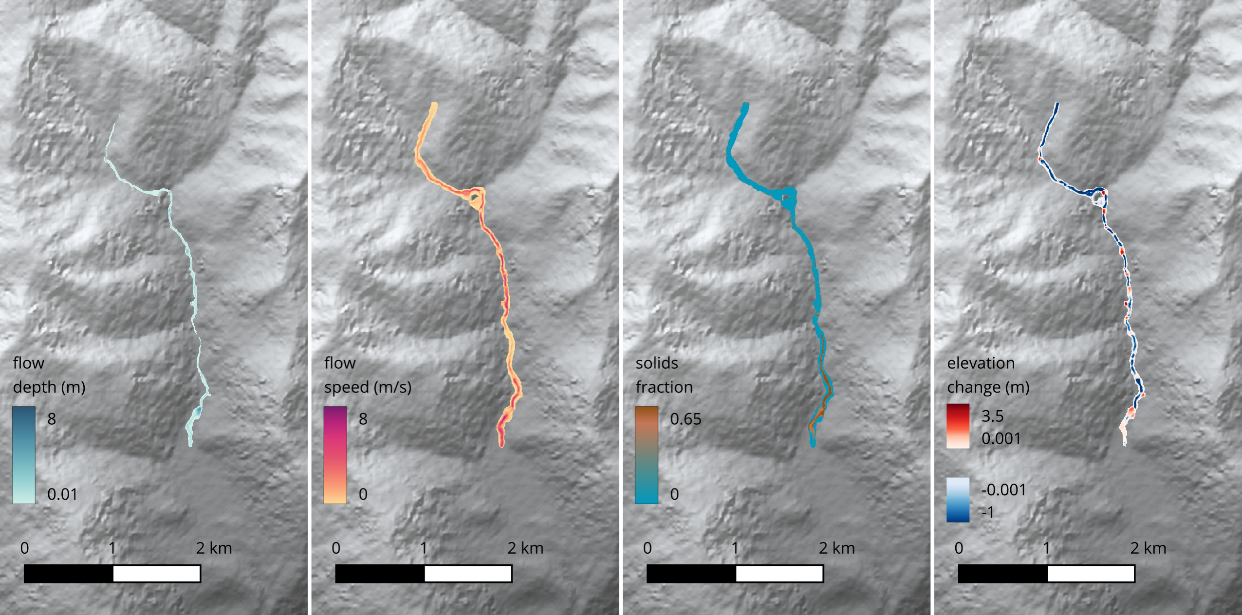
An example of the output produced by Kestrel by the Input2d_flux_SRTM.txt input file, made in QGIS (using Lahar Flow Map Tools) is shown below. (The hill shaded background map is obtained by loading the SRTM topography file separately.)

Testing

If you want to check that Kestrel is working well, there is a lightweight test suite available as a Julia script. It is unlikely to be necessary to run these if you are only using the main code branch to run simulations. However, when modifying the code, these tests can be used to identify problems.

To run all tests, change to the ./tests subdirectory and run:

$ ./julia runall.jl

Note that this assumes the existence of a valid Julia symlink within ./tests.

Most of the tests run simple simulations and perform consistency checks like verifying conservation of flow volume. They are divided into different categories that can be specified on the command line. For example to execute just the ‘noflow’ tests, which check that initially static flows with horizontal free surfaces remain at rest, you can run:

$ ./julia runall.jl noflow

Any number of test categories may be specified in this way.

The command

$ ./julia runall.jl help

prints a list of the available categories.

Warning

Running these is the first step in debugging and won’t catch everything. At this stage, you will most likely need to read runall.jl and testlib.jl carefully to understand what each test is doing.